How To Do Baseline Correction using Origin Software

Sometimes when we plot a graph of the data from an instrument, we see that the plot shifts to higher or lower values unexpectedly. These shifts across x range of data set lead to wrong analysis. This is what we know as baseline drifts. While analyzing the data, it becomes necessary to correct these drifts.

How to start

To do baseline correction using origin software, plot the graph in origin using the data you have. Now in the menu bar, click on the Analysis tab and navigate to Peaks and Baseline >> Peak Analyzer >> Open Dialog.

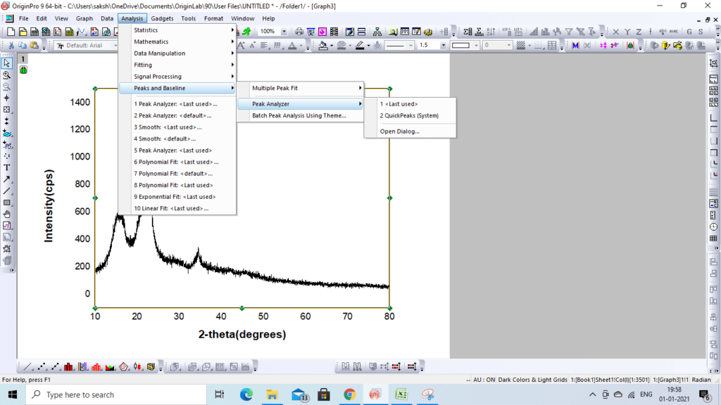
A Peak Analyzer dialogue box appears that allows users to create and subtract baselines.

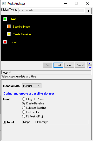
Step-1 Find the anchor points

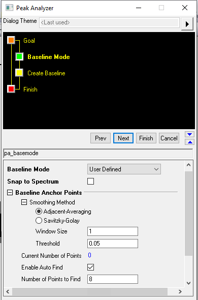
As a first step in the baseline correction, one has to find and fix the anchor points for baseline creation. There are 3 options available to find the anchor points: User-defined, XPS and End-point weighted. Different smoothing methods are available under three categories which take advantage of the relationship between the adjacent data variables.

The user-defined method allows one to create baselines using one of the following smoothing methods: – Adjacent-averaging and Savitzky-Golay.

Each smoothing point is computed from the data points within a window defined by the window size. For example for the fourth point of the data set, smoothing is done using the data points lying between (4-floor(window size/2)) and (4+floor(window size/2)). Thus, if the window size is 3, the interval will be [3, 5].

Adjacent Averaging Method

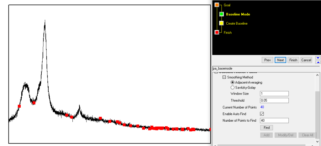
In the adjacent averaging method, each anchor point is the average of data points within the moving window. To find the anchor points, provide the value for window size and the number of anchor point you want. After this, hit the tab ‘Find’.

One needs to enter an optimal value of window size. Too big value of window size may disrupt the results.

Savitzky-Golay Method

The Savitzky-Golay filter method performs a local polynomial regression (polynomial of any order between 1 and 9) around each point and creates a new, smoothed value for each data point. This method of baseline correction is superior to adjacent averaging as it preserves the features of the data which can be “washed out” by adjacent averaging. To increase the smoothness of the result, one can increase the “window size,” or the number of data points used in each local regression.

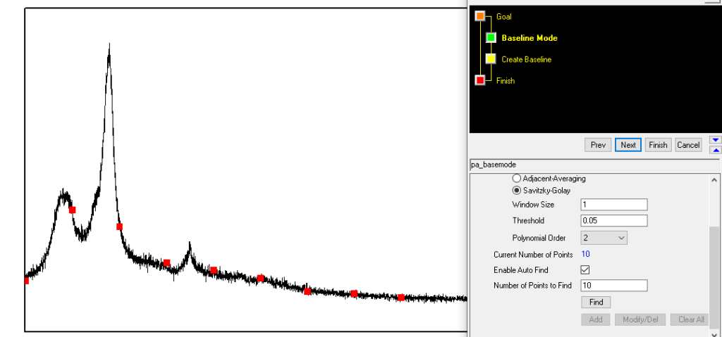
In case, the auto predictor baseline points are not satisfactory, one can modify or delete them using the Modify/Del functionality.

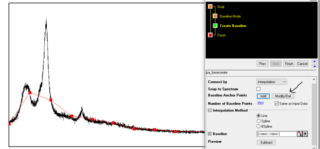
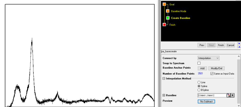
Step-2 Connect the anchor points

Anchor points can be connected either by interpolation or fitting method.

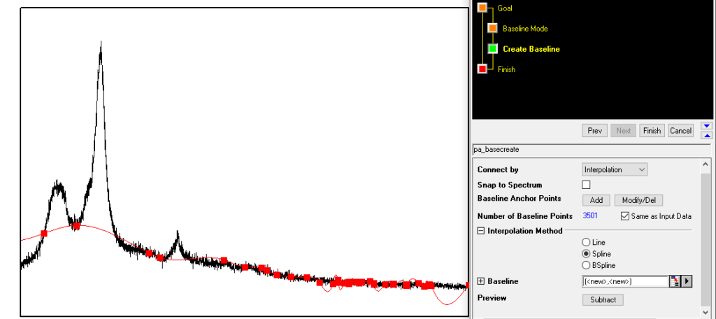
Interpolation method

One can choose either of the three methods Line, spline, and B-spline interpolation for the best results.

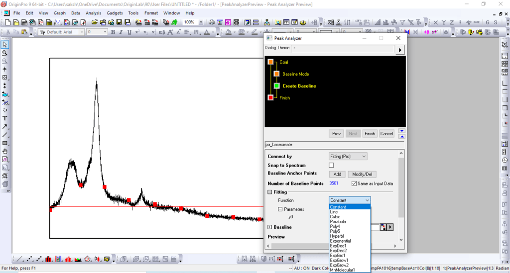
Fitting method

Several fitting options are available to connect the anchor points such as linear fitting, polynomial fitting, exponential fitting, etc. A constant line may also connect the points. Users can provide or modify the value of this constant.

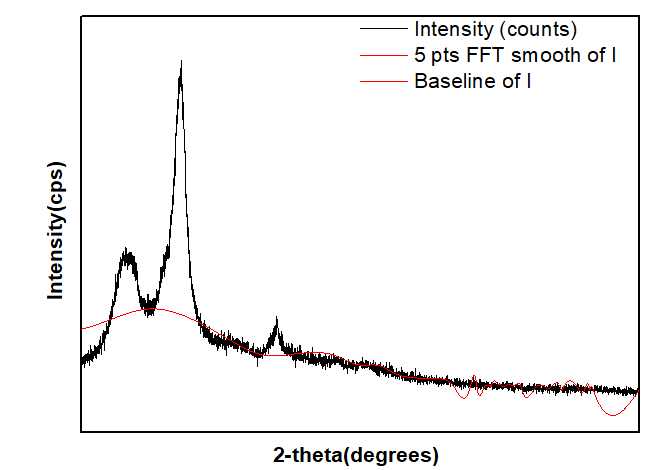
Step-3 Subtract from baseline

Data minus baseline plot looks like the graph shown in figure below.